The long view: how tax expenditures affect revenue over multiple years

This is the last of three blog posts we’re posting following the TaxDev Tax Expenditures Workshop held on 6–8 February 2023 in Kampala. This blog post is adapted from this report on tax expenditure reporting in Rwanda and Uganda.

Tax expenditure reporting is often a static exercise: the government looks at all the deviations from the benchmark system and calculates how much revenue is forgone in that year due to those deviations. The tax system is not, however, static. Taxes that allow for losses to be carried forward – the corporate income tax (CIT) and, to a lesser extent, value added taxes (VAT) – lead to provisions affecting revenue forgone over the course of multiple years. In addition, accelerated depreciation – or generous up-front capital allowances – under the CIT will also have multi-year effects, as they may lead to revenue forgone in early years, but potentially revenue gain later on, when compared with the benchmark tax system. 

Loss carry-forward

If a company makes a taxable loss in one year, it is generally able to deduct the loss from its profits in the next year. This is called ‘loss carry-forward’, and almost every CIT system in the world allows this, at least for a few years. Whilst the ability to carry forward losses is not, in and of itself, normally considered to be a tax expenditure, it can lead to forgone revenue from other provisions being ‘transmitted’ – or spread out – over time. Failing to take this into account will generally lead to revenue forgone from tax expenditures being either incorrectly estimated or allocated to an incorrect time period.

This hopefully becomes clear with an example. Consider the case of a company that made $100 in gross accounting profit (sales minus costs) in 2023. However, it posted a tax loss in 2022 and was allowed to ‘carry forward’ that loss into 2023 and subsequently deduct it from gross profits when calculating taxable profit for 2023. As a result of losses carried forward, its taxable profit in 2023 is, then, just $50. With a 20% tax rate, tax due is $10. 

Table 1: Example tax return for 2023

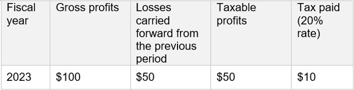
Without any additional information, it isn’t possible to identify any revenue forgone from tax expenditures in this scenario. There do not seem to be any deviations from the benchmark tax system for this company, in this year.

Consider another tax return for the same company, this time for 2022. In this year, the company again made accounting profit of $100 but also benefited from a tax credit for expenditure incurred whilst conducting research and development (R&D), of $150.

Table 2: Example tax return for 2022

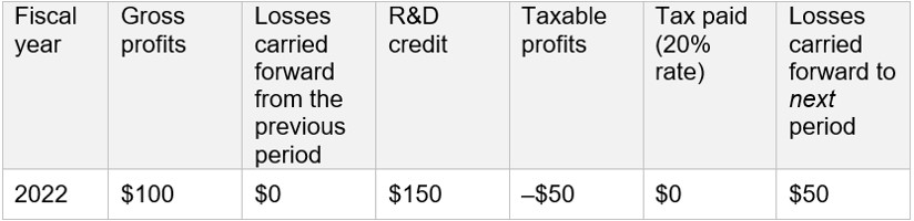
The R&D tax credit was identified as a clear deviation from the benchmark tax system, and the government wants to calculate the tax expenditure. If the R&D tax credit did not exist, then the company would have paid $20 in tax ($100×20%) in 2022. Without any additional context, it would seem as if the tax expenditure associated with the R&D tax credit is $20.

However, merging the tax returns over the two years highlights the importance of the time dimension.

Table 3: Combined tax return, 2022 and 2023

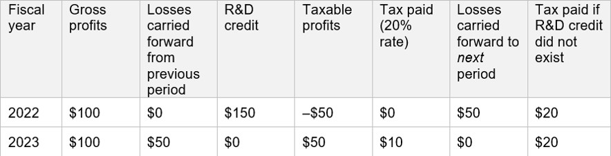
If the R&D tax credit did not exist, then the company would have paid $20 in tax in 2022. However, the company would also have paid $10 more tax in 2023, as there would not have been any loss carry-forward from the previous year. If we looked at 2022 and 2023 separately, as we did in Tables 1 and 2, we would have missed the fact that provisions in one year can affect tax paid in subsequent years.

This is not unique to R&D tax credits. Any type of CIT tax expenditure that brings a company’s taxable income position from positive to negative (such as accelerated depreciation, which is discussed below) could be transmitted over time via the loss carry-forward mechanism. Indeed, it could take many years for the effects of a tax expenditure to ‘wash out’. This would potentially also affect personal income tax (PIT), in situations where the income of unincorporated business owners is taxed in line with CIT. Most VAT systems also have a similar provision requiring net credits (where deductible input VAT exceeds chargeable output VAT) to be carried forward rather than refunded immediately.

One issue with timing differences is understanding in which year to allocate the tax expenditure. In the example above, the analyst writing the tax expenditure report for 2022 can only definitively calculate revenue forgone in 2022. Without perfect foresight, it is hard to tell how much revenue will be forgone in in 2023. For example, the company might go out of business in 2023, so it would pay zero tax regardless of whether the tax expenditure existed in 2022. Or the company might make negative gross profits in 2023 (and beyond), so would continue to pay zero tax. Tax expenditure from the credit is then not ‘realised' or reported until the company starts to post some positive level of gross profit. However, the analyst writing the tax expenditure report in 2022 cannot possibly know how the company will perform in the future.

One approach would be to assign a $20 tax expenditure to the R&D tax credit policy for the 2022 tax expenditure report, and to assign an additional $10 tax expenditure to the policy for the 2023 tax expenditure report, as the data come through. If the company instead goes out of business in 2023, or makes a further taxable loss, the tax expenditure for R&D tax credits in 2023 would be $0.

Accelerated depreciation

Another situation where timing differences affect tax expenditures is under accelerated depreciation regimes. Accelerated depreciation is when the government allows companies operating in certain sectors, or investing in certain types of assets, to depreciate the cost of the asset faster than the standard depreciation rate. Accelerated depreciation is really an issue of timing, however; companies are able to deduct the costs of their investment faster than they otherwise would have, but the total amount they are able to deduct remains the same. Accelerated depreciation is viewed as a corporate tax incentive, as companies would prefer to receive the tax deduction now rather than later. This is because companies (and people) generally prefer receiving money now over receiving it later, due to inflation and the interest they can then earn (summarised by what is termed the ‘discount rate’).

As with loss carry-forward, when calculating revenue forgone under accelerated depreciation, just focusing on a single year can hide timing effects. Consider a company that is allowed to deduct 100% of the cost of an investment in a given asset up front (also known as ‘full expensing’), when the benchmark rate of depreciation is 25% on a straight-line basis.

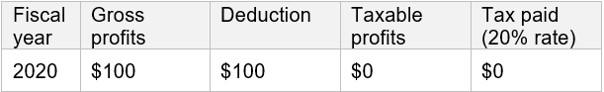
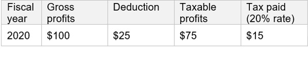
In 2020, the company makes a $100 investment that qualifies for accelerated depreciation. Whilst its gross profit is $100 in 2020, the $100 accelerated depreciation allowance has reduced its taxable profit to $0. Under the benchmark tax system, it would have had taxable profits of $75 and therefore paid $15 in tax. When writing the tax expenditure report for 2020, the analyst concludes that the tax expenditure associated with accelerated depreciation is $15, and leaves it at that.

Table 4: Accelerated depreciation and the benchmark tax system, 2020

Accelerated depreciation – 100% deduction

Benchmark system – 25% deduction

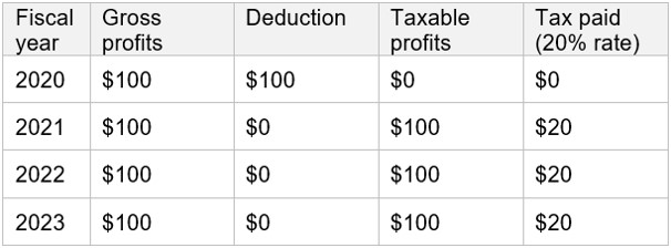
However, accelerated depreciation has important timing effects. Table 5 extends the company’s income tax returns three more years, under both the 100% deduction and the 25% deduction.

Table 5: Accelerated depreciation and the benchmark tax system, 2020 to 2023

Accelerated depreciation – 100% deduction

Benchmark system – 25% deduction

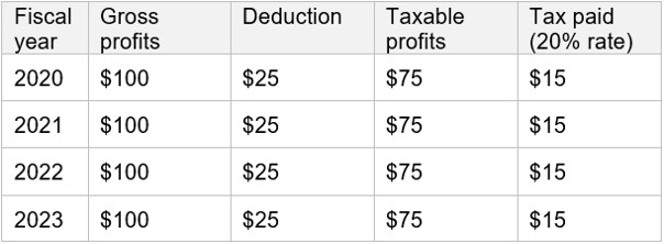
Under the benchmark tax system, the cost of the investment is spread out over four years. This means that with accelerated depreciation, although the company pays $15 less tax in 2020 than in the benchmark system, it pays $5 more for each of the three years after that. The total revenue forgone to the government is therefore zero, when looking over the whole four-year period (though this is not true when adjusting for the discount rate – like companies, governments would prefer to have the tax revenue sooner rather than later).

As with loss carry-forward, the lack of perfect foresight means that the analyst cannot predict the true revenue forgone in 2021 and beyond – it depends on whether the company goes out of business, makes taxable losses, etc. in the subsequent three years. An analyst can look backwards, however, and see how previous provisions affect tax expenditure today. For this company, this would mean assigning a revenue forgone of $15 in the 2020 tax expenditure report. As the data come in for 2021, the analyst would assign a revenue gain (or negative tax expenditure) of $5 for the 2021 report, and so on for subsequent years.

Complexity and data requirements

Unfortunately, incorporating the timing effects of tax expenditures increases the time taken to calculate tax expenditures. For example, using Tables 1 and 2, tax expenditures from the R&D tax credit were relatively easy to calculate. In Table 3, we had to simulate how the loss carry-forward would change in the absence of the R&D tax credit, after one year. With multiple years, multiple provisions and potentially incomplete return data, this can become complex.

Timing differences arising from accelerated depreciation are potentially even more complex, as different classes of assets (plant and machinery, computers, buildings, etc.) might have different rates of accelerated depreciation and different benchmark rates, and a company may own a mix of all these types of assets. Even without incorporating the timing effects of accelerated depreciation, the analyst would have to have information on depreciation allowances claimed for each class of assets that share the same accelerated and benchmark depreciation rates. In many developing countries (and often in developed countries), this level of detail is not available from tax returns.

To account for timing effects, the analyst would at least need information on the net-of-depreciation value of assets, and depreciation allowances claimed, for each asset class. They would then have to simulate counterfactual tax paid if the benchmark depreciation schedule had been used, instead of accelerated depreciation. A report by the OECD provides more detail on this calculation.

It is not always possible to incorporate all of the effects discussed above and it is certainly not possible to tell the future. However, an awareness of these issues and how they might manifest in revenue forgone calculations can help to provide a more accurate estimate of revenue forgone or a better understanding of the limitations of approaches currently taken.